Your Demand Forecast Is Only as Good as the Architecture Behind It

Have you ever sat in a planning meeting where someone pulled up a forecast and nobody in the room fully trusted it?

That question sits at the Centre of most demand planning failures. Not the data. Not the model. The trust. And trust in a forecast breaks down when the architecture underneath it is held together with spreadsheets, manual exports, and disconnected systems.

I want to walk you through how we think about demand forecasting at Infocepts, not as a data science exercise, but as a business infrastructure problem. We have implemented this across retail, manufacturing, CPG, pharma, and telecom. The business context changes. The core principle stays the same: if your forecast cannot answer a business question in plain language, it is not working hard enough.

Here is the full architecture and what it looks like when it runs on Databricks with an Agentic AI layer on top.

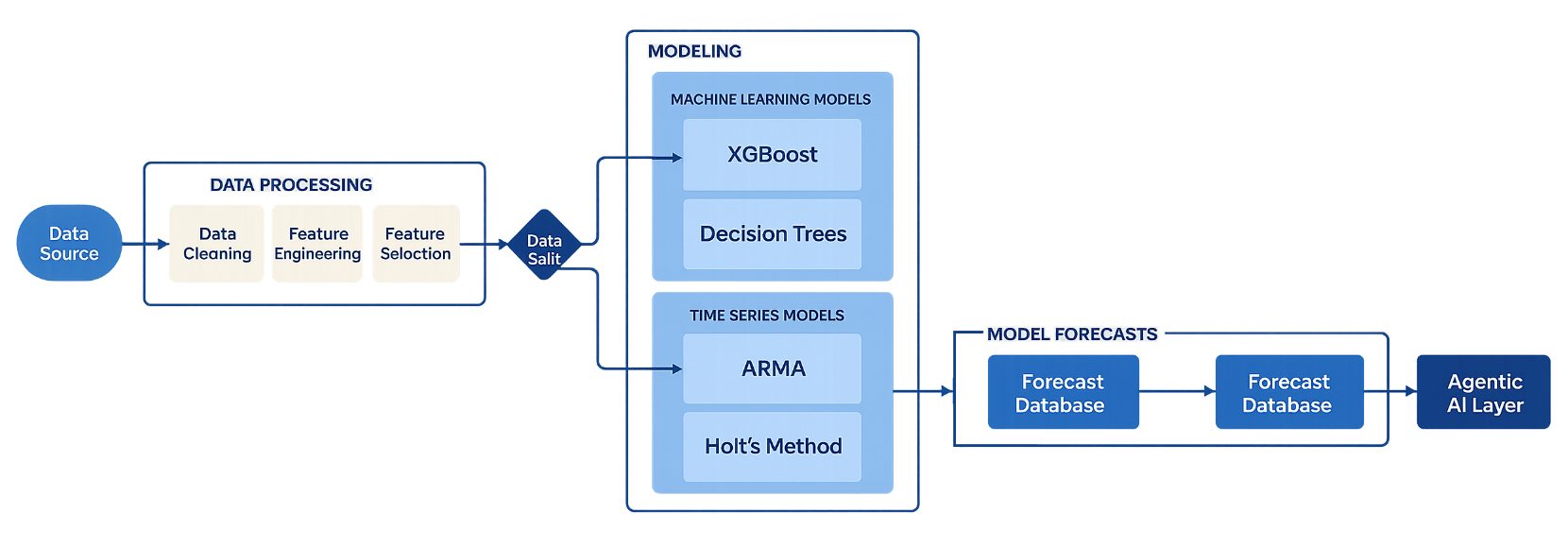
Figure 1: End-to-end demand forecasting architecture-from sales data sources through data preparation, ML modeling, forecast database, and the Agentic AI layer.

With the Business Question, Not the Data

Most demand forecasting projects start in the wrong place. They start with the dataset. The right place to start is with the person who has to make a decision and ask: what do they need to know, at what level of detail, and how often?

Take a manufacturing firm managing spare parts across multiple regions and plants. The sales team visits distributors monthly. That one fact tells you everything about the required forecast grain: monthly forecasts at the SKU-region level. Not daily. Not at a product family rollup. Monthly, by SKU, by region.

That grain decision drives every downstream choice – how you aggregate data, how you structure your model, and how you evaluate whether the forecast is useful. Get it wrong and you can have a technically accurate model that the business ignores because it does not answer the question they are actually asking.

The granularity of your forecast is not a data science decision. It is a business decision. The data science follows from it.

The Data Foundation: Building the Dataset

When we build a demand forecasting solution, we work with both internal business data and external macro signals. Internal data covers sales history, promotions, regional demand patterns, and SKU-level performance. External data brings in inflation, wage levels, unemployment rates, and seasonality – anything that affects buying behavior but sits outside the four walls of the business.

For this manufacturing scenario, we simulate data across start dates, end dates, regions, plants, and product categories. The simulation includes holiday effects, seasonality cycles, promotional uplift, and macroeconomic inputs. The resulting dataset mirrors what a real manufacturing firm would bring to the table.

Below is what that dataset looks like – 74,400 rows spanning SKUs, regions, plants, demand units, prices, promotions, macroeconomic signals, and lagged demand features.

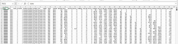
Figure 2: Simulated manufacturing demand dataset-columns include date, SKU, region, plant, demand units, price, promotion flags, macro indicators, and lagged demand features.

Loading the Data into Databricks

The data is stored as a CSV and loaded into a Databricks notebook via a defined file path in the workspace. A simple loaddata() function reads the CSV using pandas and returns a clean DataFrame for all downstream steps.

Figure 3: File path pointing to the synthetic manufacturing demand dataset in the Databricks workspace.

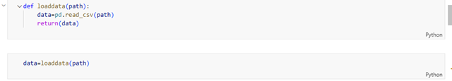
Figure 4: loaddata() function—reads the CSV from the defined path and returns a pandas DataFrame.

Why Unity Catalog Is Central to This Architecture

Once the data is loaded, it goes into Unity Catalog – Databricks’ centralized governance layer. Unity Catalog manages access control, data lineage, auditing, and discovery across the full data lakehouse. Tables, views, files, and ML models all live under unified governance.

For demand forecasting, this matters for two reasons. First, forecast data is commercially sensitive – Unity Catalog handles permission enforcement at the asset level. Second, the Agentic AI layer we build on top needs to read that data securely, with full semantic understanding of what each column means. Unity Catalog provides the metadata infrastructure that makes the agent reliable, not just functional.

Data Preparation: The Unglamorous Work That Determines Accuracy

The quality of your forecast is determined in data preparation, not in model selection. Two issues show up in almost every dataset we work with.

First, here is what the summary statistics look like across the key fields – 74,400 records, demand units ranging from 0 to 2,426, prices from $28.95 to $112.69, and a full set of lagged demand and rolling mean features.

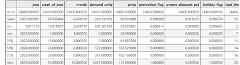
Figure 5: Summary statistics across the dataset—count, mean, standard deviation, minimum, 25th/50th/75th percentiles, and maximum for demand units, price, promotion, holiday, and lead time fields.

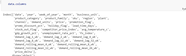
Figure 6: Full column index of the dataset—includes SKU hierarchy, macro signals (GDP growth, unemployment, FX index), demand lags (1 week through 52 weeks), and rolling means (4 weeks through 26 weeks).

Missing Values

Missing values are the most common data quality problem in demand forecasting. Most ML algorithms cannot handle them natively, so they have to be addressed before modeling begins. Where a missing value genuinely represents zero demand – no orders placed, no sales recorded – we fill with zero. Where it is a data collection failure, we use imputation. The distinction matters and takes judgment, not just code.

Below is the function we use to check for and impute missing values. We check counts first, then fill all null values with 0 using fillna().

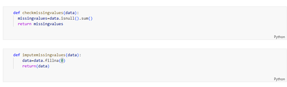
Figure 7: checkmissingvalues() identifies null values by column; imputemissingvalues() fills them with 0 using pandas fillna().

Outliers

Outliers in regression-based forecasting can significantly distort model outputs. A single unusually large order – a bulk purchase, a data entry error – can shift a model’s entire prediction range if not addressed.

We use the interquartile range method: calculate Q1 and Q3, compute the IQR as the difference, and flag any value outside Q1 minus 1.5x IQR or Q3 plus 1.5x IQR as an outlier. Those flagged values are substituted with the column median. Conservative, interpretable, and effective.

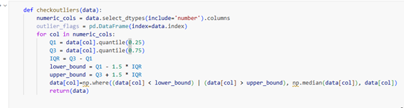
Figure 8: checkoutliers() identifies numeric columns, computes IQR bounds (Q1 ± 1.5×IQR), and replaces outlier values with the column median using np.where().

The Machine Learning Pipeline: Where the Forecast Gets Built

Demand forecasting is a time series problem. The core decision before you touch any algorithm is whether to build a global model – one model for all SKUs – or individual models per SKU or SKU-region combination.

Global Model vs. Per-SKU Models

A global model is operationally simpler. But if order quantity varies from near-zero to 200,000 across different SKUs, a single global model will underfit high-variance products and overfit stable ones. Per-SKU models capture that variance. They are more accurate when data supports them. The trade-off is maintenance complexity at deployment.

In this manufacturing scenario, we train individual models for each SKU-region combination. That level of granularity matches the business requirement. You will need to determine what matches yours – sometimes that only becomes clear through testing both approaches on your actual data.

Train-Test Split: Avoiding the Leakage Problem

Time series data has a constraint that cross-sectional data does not: you cannot allow future observations to inform past predictions. A random split on time series will create data leakage – your model learns from the future and reports falsely high accuracy. We use date-based filtering to enforce a clean temporal boundary. Non-negotiable.

Algorithms We Run in Parallel

For each SKU-region combination, we run four regression algorithms and select the best performer on held-out test data:

• Random Forest – handles nonlinear relationships and feature interactions; robust to outliers
• Lasso Regression – performs automatic feature selection by penalizing less predictive variables
• Linear Regression – provides a clean, interpretable baseline
• Ridge Regression – manages multicollinearity when predictors are correlated

The code below shows the model loop in action – iterating through each region-SKU combination, fitting all four models, evaluating on validation data via RMSE, selecting the best model, and storing predictions alongside model name and error metrics.

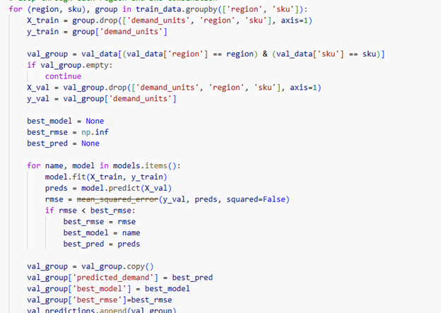
Figure 9: Per-SKU model training loop—iterates through region-SKU combinations, fits Random Forest, Lasso, Linear Regression, and Ridge models, selects the best based on RMSE on validation data, and stores predictions.

The winning model – selected by accuracy on test data – has its parameters saved per SKU-region combination. When new data arrives the following month, we retrieve those stored parameters and run inference on the updated dataset. No retraining required until the data distribution shifts enough to warrant it.

Stored model parameters mean your January forecast run is a retrieval and inference operation – not a full retraining cycle. That matters for both speed and operational reliability at scale.

The Agentic Layer: Where the Forecast Starts Talking Back

This is where the architecture goes from useful to genuinely different.

Once the forecast outputs are stored as tables in Unity Catalog, we build an Agentic AI layer on top of them. The agent connects a large language model to the governed forecast data, giving it the ability to read demand figures, inventory positions, and confidence intervals through SQL – with full semantic understanding of what those fields mean in the business context.

The result: a business user can type a plain-language question and get a direct, accurate answer.

“Which SKUs are likely to stock out next month in the Southwest region?” – that question, typed into a chat interface, returns a table, a chart, and a ranked list. No SQL. No analyst in the middle. No waiting until Thursday.

How We Build the Agent in Three Steps

1. Govern and enrich the forecast data in Unity Catalog. Add business metadata – SKU hierarchy, region mapping, calendar attributes, column descriptions. The agent needs semantic context, not just raw column names, to reason accurately. 
2. Define the intent library. Identify the twenty or thirty business questions that planning, operations, and commercial teams ask repeatedly. These become the agent’s reasoning blueprint – the queries it is optimized to answer reliably. 
3. Build the tool-enabled agent on Databricks. The agent uses SQL execution, table lookup, and metric calculation tools to translate natural-language questions into validated queries against Unity Catalog. Iterate on prompt tuning and metadata enrichment until the agent’s accuracy on real business questions reaches a trustworthy threshold. 

Over time, logged interactions feed back into prompt refinement. The agent gets more accurate with use, not less. That compounding improvement is one of the most underappreciated benefits of the Agentic architecture.

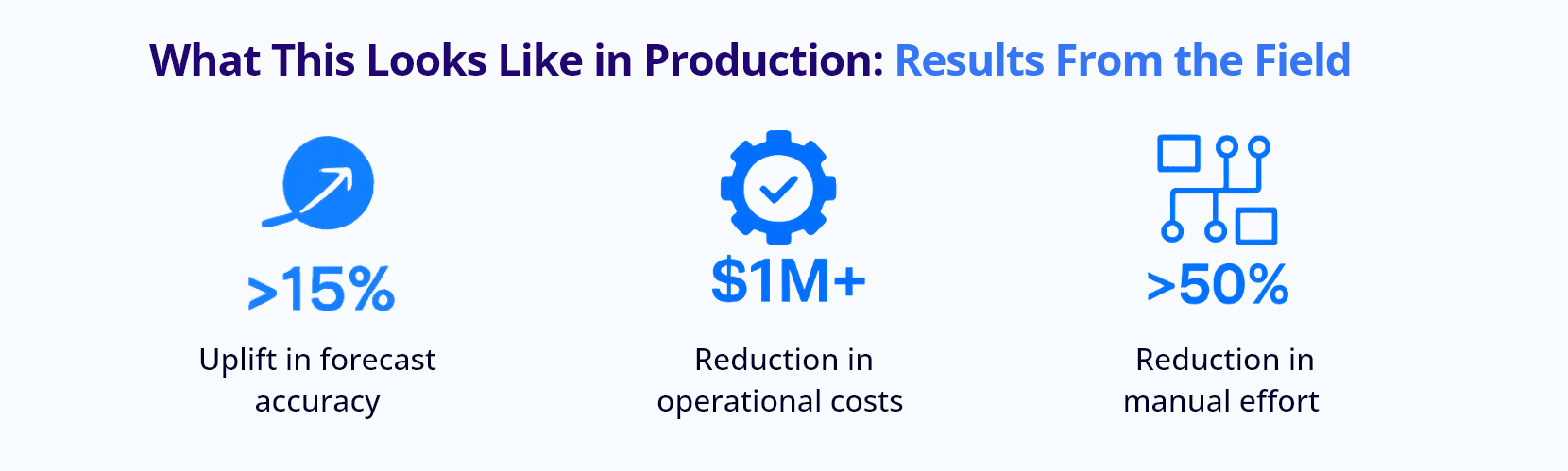
What This Looks Like in Production: Results From the Field

We have implemented this architecture for clients across manufacturing, retail, CPG, pharma, and telecom. The business context varies. The outcomes do not vary much.

For a manufacturing client running this full stack – ML-based demand forecasting on Databricks with Agentic AI on top – here is what the numbers looked like:

>15%	Uplift in forecast accuracy compared to the previous business forecasting process — directly translating to better production planning and inventory decisions.

$1M+	Reduction in operational costs through improved planning accuracy. Better forecasts mean less emergency procurement, less overstock, and fewer missed deliveries.

>50%	Reduction in manual effort through automation of the forecasting pipeline — from data ingestion through model selection, inference, and reporting.

Beyond the numbers: on-time delivery improved. Customer satisfaction scores moved. The operations team stopped spending Monday mornings reconciling last week’s forecast against actuals and started using that time to act on what the forecast was telling them.

That shift – from reconciling the past to acting on the future – is what a well-built demand forecasting architecture is supposed to produce.

Where This Goes Next: Supply Chain as a Full System

Demand forecasting is one input into a supply chain. Infocepts is extending this architecture into a full supply chain optimization layer – where the same Databricks foundation and Agentic AI interface that answers demand questions also answers inventory tracking questions, stock-out risk questions, and supplier performance questions.

The manufacturing use case in this blog is the starting point, not the ceiling.

The Bottom Line

If your planning team does not trust your forecast, the model is not the problem. The architecture is.

A demand forecasting system built on Databricks – with proper data governance in Unity Catalog, a rigorous ML pipeline that selects the right model per SKU-region combination, and an Agentic AI layer that answers business questions in plain language – changes how an organization makes decisions. It does not just produce a number. It produces confidence.

We have done this across industries. The data changes. The methodology holds.

If your current forecasting process involves spreadsheet handoffs, weekly reconciliation meetings, or a planning team that spends more time arguing about the forecast than acting on it – let’s talk. Visit infocepts.ai to start the conversation.